Lab 7 - Relevance Ranking#
Th. 14.11.2024 15:00-17:00
1 - Term Frequency - Inverse Document Frequency (TF-IDF)#
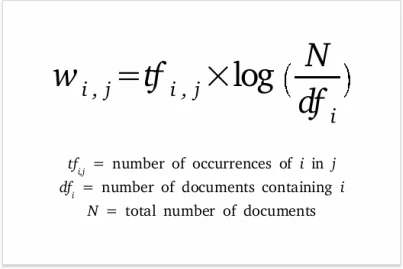
\( TF-IDF(t,d,D) = Term Frequency (t,d) \times Inverse Document Frequency (t,D)\)

## the data set is again from Seattle Airbnb Open Data on Kaggle
## https://www.kaggle.com/datasets/airbnb/seattle
## including full descriptions of airbnb listings and average review score

import pandas as pd
listings = pd.read_csv('listings.csv')
1.1 - Data Preprocessing#
## select the columns of interest and drop all rows containing missing values
listings_selected = listings[['id','name','neighborhood_overview','neighbourhood_group_cleansed']].dropna()

## rename a column
listings_selected = listings_selected.rename(columns={'neighbourhood_group_cleansed':'neighborhood'})
listings_selected
## group and aggregate overviews by neighborhood
grouped_df = listings_selected.groupby('neighborhood')['neighborhood_overview'].agg(lambda x: ' '.join(x)).reset_index()
grouped_df
import spacy
nlp = spacy.load("en_core_web_sm")

## function to keep only alphabetical terms (excluding stop words) in the overview
def clean_text(text):
    doc = nlp(text)
    alpha_non_stop_tokens = [token.text for token in doc if token.is_alpha and not token.is_stop]
    cleaned_text = ' '.join(alpha_non_stop_tokens)
    return cleaned_text

## apply the function to the overview column
grouped_df['cleaned_overview'] = grouped_df['neighborhood_overview'].apply(clean_text)
grouped_df
1.2 - Compute TF-IDF#
## compute TF-IDF using packages sklearn
from sklearn.feature_extraction.text import TfidfVectorizer
tfidf = TfidfVectorizer()
# compute TF-IDF on the 'cleaned_overview' column
tfidf_matrix = tfidf.fit_transform(grouped_df['cleaned_overview'])

## convert TF-IDF matrix into a dataframe
tfidf_df = pd.DataFrame(tfidf_matrix.toarray(), columns=tfidf.get_feature_names_out())

# set the 'neighborhood' column as the index in the dataframe
tfidf_df.set_index(grouped_df['neighborhood'], inplace=True)

tfidf_df
1.3 - Extract top TF-IDF results for one neighborhood#
## extract one neighborhood as a dataframe, transpose it, and reset column name
tfidf_ballard = tfidf_df.loc[['Ballard']].drop('neighborhood', axis=1).transpose()
tfidf_ballard.columns = ['TF-IDF']

## sort the tfidf values and only show the top 20 results
tfidf_ballard = tfidf_ballard.sort_values('TF-IDF', ascending=False)
tfidf_ballard.head(20)
1.4 - Relevance Ranking with TF-IDF#
With TF-IDF for each word in the document, we can then compute the relevance of a query in respect to the candidate documents.
## given two query terms
from sklearn.metrics.pairwise import cosine_similarity
query_terms = ['pike', 'coffee']

## combine the query terms into a single string
query = ' '.join(query_terms)

# add the query string to the dataframe as a new row
new_row = {'neighborhood': 'query_term',
           'neighborhood_overview': '',
           'cleaned_overview': query}
query_df = pd.DataFrame([new_row])
grouped_query_df = pd.concat([grouped_df, query_df], ignore_index=True)

# compute TF-IDF for both documents and query
tfidf_vectorizer = TfidfVectorizer()
tfidf_matrix = tfidf_vectorizer.fit_transform(grouped_query_df['cleaned_overview'])

# get the TF-IDF vector for the query
query_tfidf = tfidf_matrix[-1]

# calculate cosine similarity between query TF-IDF and documents
cosine_similarities = cosine_similarity(tfidf_matrix[:-1], query_tfidf.reshape(1, -1))

# get the top three most relevant neighborhoods given query terms
top_indices = cosine_similarities.flatten().argsort()[-3:][::-1]
grouped_df['neighborhood'].iloc[top_indices]
2 - Submission#
Run the codes above, explore TF-IDF results for different neighborhoods and try different query terms.
Complete the following part and submit the .ipynb file on Moodle.
What are your option of query terms and their top 3 most relevant neighborhoods:
Query terms:
Top 3 most relevant neighborhoods:
Whether the results make sense to you:
…
